Dendritic nonlinearities are tuned for efficient spike-based computations in cortical circuits
- University of Cambridge, United Kingdom
- Hungarian Academy of Sciences, Hungary
- MRC Laboratory of Molecular Biology, United Kingdom
- Janelia Farm Research Campus, Howard Hughes Medical Institute, United States
- University College London, United Kingdom
- Central European University, Hungary
Figures
Figure 1 with 3 supplements

Spike-based implementation of analogue computations in neural circuits.
(A) Computation (top) is formalized as a mapping, , from presynaptic activities, (left), to the postsynaptic activity, (right). As neurons communicate with spikes, the implementation (bottom) of any computation must be based on the spikes the presynaptic neurons emit, (middle). Optimal input integration in the postsynaptic cells requires that the output of is close to that of . (B) The logic and plan of the paper. Grey box in the center shows theoretical framework, blue boxes around it show steps necessary to apply the framework to neural data. To compute the transformation from stimulation patterns (bottom left) to the optimal response (bottom right) we assumed linear computation (top right) and specified the presynaptic statistics based on cortical population activity patterns observed in vivo (top left). To demonstrate the validity of the approach, we studied the fundamental qualitative properties of the optimal response (Figure 2), compared it to biophysical models (Figures 3–4) and tested it in in vitro experiments (Figure 5). (C) The optimal postsynaptic response (purple line, bottom) linearly integrates spikes from different presynaptic neurons (top: rasters in shades of green; middle: membrane potential of one presynaptic cell) if their activities are statistically independent. (D) Optimal input integration becomes nonlinear (purple line, bottom) if the activities of the presynaptic neurons are correlated (rasters in shades of green, top), even though the long-term statistics and spiking nonlinearity of individual neurons remains the same as in (C). In this case, the best linear response (black line, bottom) is unable to follow the fluctuations in the signal.
Figure 1—figure supplement 1
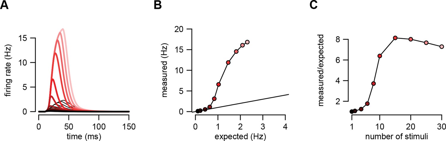
An example of supralinear input integration with firing rate-based rather than membrane potential-based computations.
(A) Optimal response (dark red to pink) and linear predictions (black) to an increasing number of input spikes (130) arriving with a short delay (1 ms). Throughout the paper, we assumed that the variables relevant for the postsynaptic neurons were the sub-threshold membrane potential values of their presynaptic partners, and for consistency, that the function the postsynaptic neuron computed was also represented by its sub-threshold membrane potential. We chose membrane potentials as the time-dependent representational substrate because they can be directly measured and are well defined at all times in individual trials in electrophysiological experiments (in contrast to firing rates which require averaging over trials or time). Here, we demonstrate that our basic results apply equally if computations are instead based on firing rates. We used the same model of presynaptic statistics as before but defined the intended computation as a linear mapping between pre- and postsynaptic firing rates (cf. Equation 5): where is the firing rate of presynaptic neuron as defined previously. This means that the optimal spike-based implementation is (cf. Equation 6): . Therefore, based on this equation, the equations of assumed density filtering (Equations 20–22) remained unchanged but the optimal response was computed as where is the posterior mean firing rate of neuron in population state , as before. Here we plot as the optimal response. (B) The amplitude of the measured response as a function of the linear expectations. (C) Nonlinearity of the response amplitude as a function of the number of input spikes. The nonlinearity in this case is comparable to that obtained in the case of membrane potential-based computations (cf. Figures 2 and 5 of the main text). In fact, it is even stronger because the firing rate is a highly supra-linear (here: exponential) function of the membrane potential. Parameters were tuned to hippocampal sharp wave dynamics (Table 1, HP) with , , and .
Figure 1—figure supplement 2
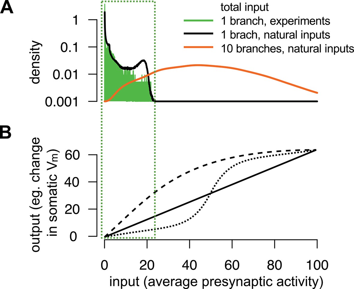
The range of total dendritic inputs in vitro and in vivo.
(A) Input ranges to a single dendritic branch in our in vitro experiments (green histogram) are similar to the input ranges expected during natural, in vivo stimulus conditions (black curve). Throughout the paper, we assumed that the dynamics of the postsynaptic cell is governed by the total input arriving to the cell, (cf. Equation 6): where is the average of the estimated presynaptic membrane potentials. To illustrate the input distribution in our in vitro cortical experiment (green histogram), we computed the values of the total input for that were the stimuli given to the cell shown in Figure 5B–C and, just as in Figure 5C–E, we used neocortical input statistics (Table 1, NC) to determine . Next, to compute the input distribution to a dendritic branch relevant in vivo (black curve), we simulated 100 s of activity from a presynaptic population of neurons undergoing dynamics with the same neocortical statistics and estimated in a similar way, but now with being the spikes generated using these in vivo statistics. We observed an excellent overlap between the ranges spanned by the two distributions suggesting that the relatively simple stimuli used in our in vitro experiments were appropriate to probe the physiologically relevant integrative properties of a single dendritic branch. However, note that the range of the input received in vivo by a whole neuron (orange curve), rather than a single branch, can be substantially wider than that probed in our experiments. We modelled the neuron as possessing 10 branches receiving statistically independent inputs, with the total input being an average across all synapses and branches. (B) Examples for single neuron computation, . Note, that although can be highly nonlinear over the whole-neuron input range (orange distribution in A), in many cases it can be reasonably well approximated by a linear function over the single-branch input range used in our in vitro experiments (green box).
Figure 1—figure supplement 3

Nonlinear computation.
(A) To demonstrate that the theory applies to the case when the computation is nonlinear, we assumed that the postsynaptic neuron computes a sigmoidal function of the weighted sum (specifically the average) of the presynaptic membrane potentials (cf. Equation 5): where and are the threshold and the slope of the sigmoidal nonlinearity, respectively (see inset, which also shows the marginal distribution of the inputs). To demonstrate the need for nonlinear dendritic integration, we compared the optimal response (black, Equation 3, where is defined above, and the posterior is approximated by Equations 20–22) with a response of a linear model (grey), a model with nonlinear soma but linear dendrites (somatic, orange; Equation 31) and the clustered dendrite model with nonlinear dendrites and nonlinear soma (clustered, red). For the somatic nonlinearity, we chose a sigmoidal function to match the form of the required computation and fitted its parameters to training data. For the clustered dendrite model, the dendritic nonlinearities were fitted to the data but the somatic nonlinearity was assumed to be identical to the nonlinearity used for the computation, . We cross-validated the quality of the fits on a separate set of test data. Similar test and training errors confirmed that the parameter optimisation found good, locally near-optimal solutions without significant overfitting (not shown). (B) The error (mean sd, Equation 33) of the clustered dendrite model (red) is similar to the error of the optimal response (black) and is substantially smaller than the error of the models with linear dendritic integration (grey and orange). Moreover, having a global nonlinearity does not provide substantial improvement over the purely linear response, further emphasising the importance of nonlinear dendritic integration. Parameters were Hz, Hz, mV, ms, mV, mV, Hz, mV, ms, , and mV.
Figure 2 with 1 supplement
Nonlinearities in the optimal response.
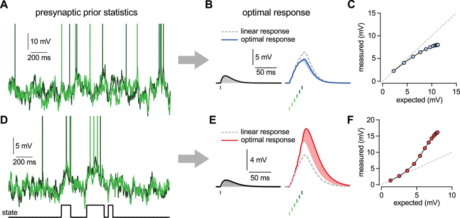
(A–C) Second order correlations between presynaptic neurons (A) imply sublinear integration (B–C). (A) Membrane potentials and spikes of two presynaptic neurons with correlated membrane potential fluctuations. (B) The optimal response (solid line) to a single spike (left) and to a train of six presynaptic spikes (right, green colors correspond to different presynaptic cells, two of which are shown in A) when the long-run statistics of presynaptic neurons are like those shown in (A). Shaded areas highlight how response magnitudes to a single spike from the same presynaptic neuron differ in the two cases: the response to the sixth spike in the train (right, light blue shading) is smaller than the response to a solitary spike (left, gray shading) implying sublinear integration. Dashed line shows linear response. (C) Response amplitudes for 1–12 input spikes versus linear expectations. (D–F) Same as (A–C) but for presynaptic neurons exhibiting synchronized switches between a quiescent and an active state, introducing higher order correlations between the neurons (D, bottom). In this case, the optimal response shows supralinear integration (E–F).
Figure 2—figure supplement 1
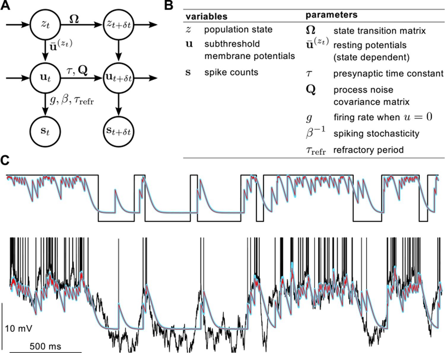
Definition of the statistical model describing presynaptic activities and illustration of the inference process in the model.
(A) Graphical model showing statistical dependencies between variables (quantities changing in time, circles), and the parameters (quantities constant on the time scale of our interest, above and beside arrows) controlling those dependencies. (B) Table showing the variables and parameters of the model. See Materials and methods for further details. (C) Validating assumed density filtering (Equations 20–22) with one presynaptic cell and two states. Black shows the true state variable (top), and membrane potential trace with the spikes indicated by vertical lines (bottom). Cyan shows the posterior mean state variable (top) and membrane potential (bottom) obtained by assumed density filtering, red shows the corresponding posterior means estimated by particle filtering. Parameters were , mV, ms, Hz, mV, mV and Hz.
Figure 3 with 2 supplements
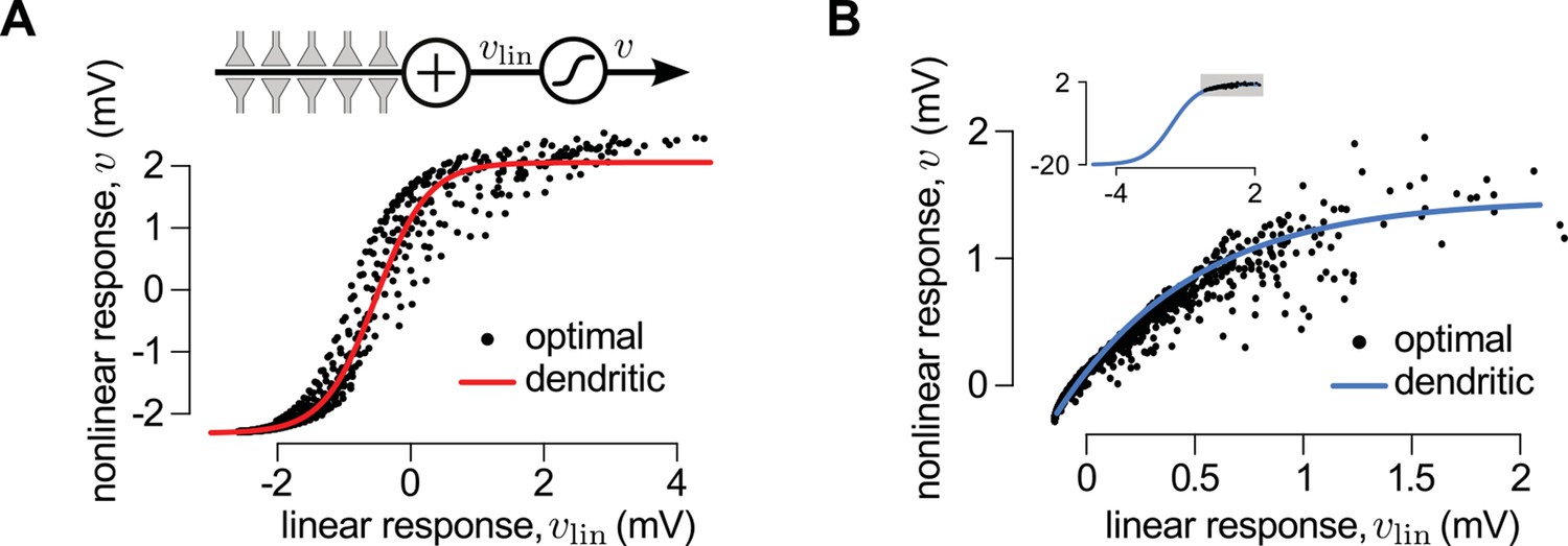
A canonical model of dendritic integration approximates the optimal response.
(A) The optimal response (black) and the response of a canonical model of a dendritic branch, (inset), with a sigmoidal nonlinearity (red, Equation 25) as functions of the linearly integrated input, (inset, Equation 24), when the presynaptic population exhibits synchronized switches between a quiescent and an active state, as in Figure 2D. Black dots show optimal vs. linear postsynaptic response sampled at regular ms intervals during a s-long simulation of the presynaptic spike trains. (B) Optimal response (black) approximated by the saturating part of the sigmoidal nonlinearity (blue) when the presynaptic population is fully characterized by second-order correlations, as in Figure 2A. Inset shows the same data on a larger scale to reveal the sigmoidal nature of the underlying nonlinearity (gray box indicates area shown in the main plot).
Figure 3—figure supplement 1
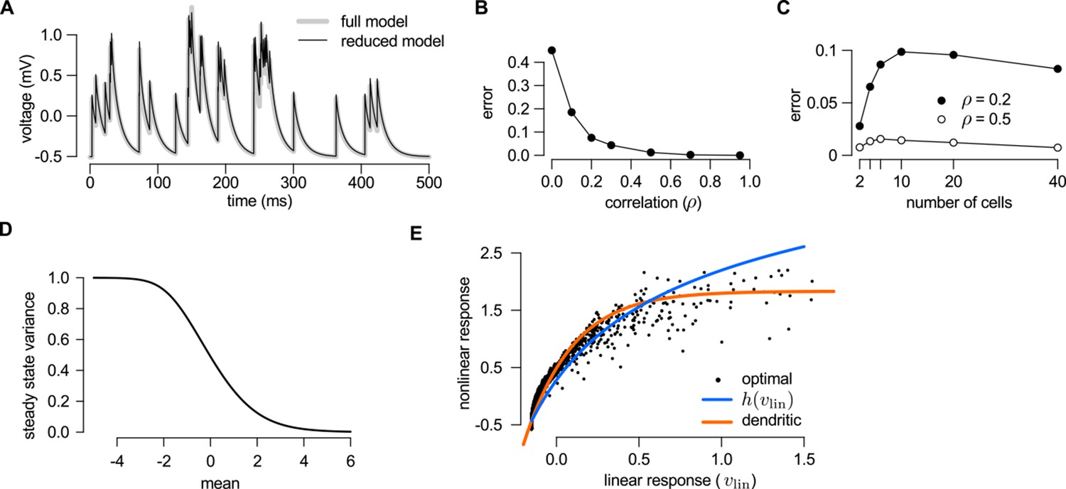
Reducing the optimal response with second order correlations to a canonical model of dendritic integration.
(A–C) Comparing the full (Equations 20–23) and the reduced model Equations A99-A100) of the optimal response. The estimates of the mean presynaptic membrane potential by the full model (A, grey) and the reduced model (A, black) are nearly identical. The error of the reduced model (quantified as the mean squared difference between the two models normalized by the variance of the full model) decreases monotonically with increasing correlations in the presynaptic population (B) and remains bounded as the number of neurons increases (C). (D) Steady state posterior variance, , as a function of the posterior mean, , in the reduced model (Equation A100). (E) Comparing the linear-nonlinear model and the optimal response. Black dots: the optimal response against the output of the linear model, (Equation 24). Blue line: sigmoidal nonlinearity operating in the linear-nonlinear model at the arrival of spikes, (Equation A103). Orange line: the result of numerically fitting a sigmoidal nonlinearity in the canonical model (Equation 25) to the optimal response. Parameters were , Hz (A–C), or , Hz (D–E), and mV, ms, mV (A–E), and (A) or as indicated on the x-axis (B) or in the legend (C). For details, see Appendix B.
Figure 3—figure supplement 2
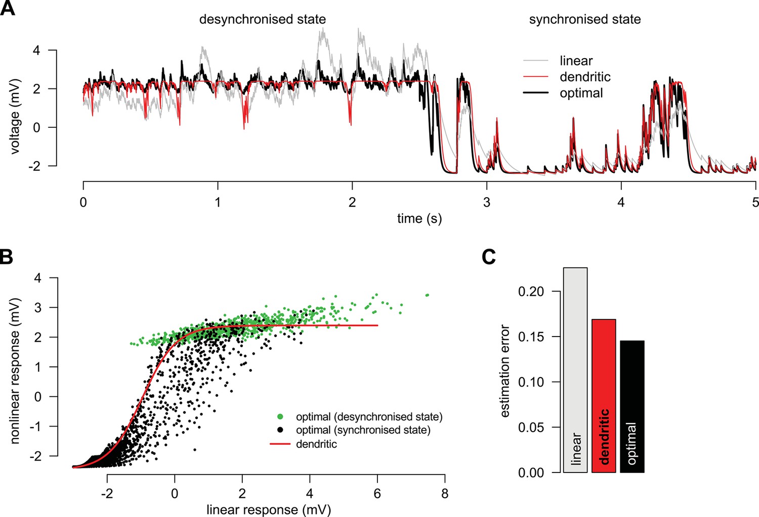
Adaptation without parameter change.
(A) We simulated a presynaptic population with two different global activity states, a synchronized and a desynchronized state and first determined the optimal response in the two states separately (black). Next, we trained a linear (grey) and a nonlinear (red) dendrite to approximate the optimal response in both the synchronized and the desynchronized state (grey). (B) Green and black dots indicate the optimal response as a function of the best linear response respectively during the desynchronized and synchronized states. The same single dendritic nonlinearity (red line) can efficiently approximate the optimal response in both states simply because each state uses a different part of the input range of this nonlinearity: during the synchronized state the expansive supralinearity of the upstroke is being predominantly used, while during the desynchronized state the saturating sublinear-linear regime is dominating the response. (C) The error of the dendritic response is slightly larger than that of the optimal response but still substantially smaller than the error of the linear response. Parameters of the synchronized state were Hz, Hz, mV, ms, mV, mV, Hz, mV, ms and and the desynchronized state was identical to a persistent active phase of the synchronized state.
Figure 4 with 2 supplements
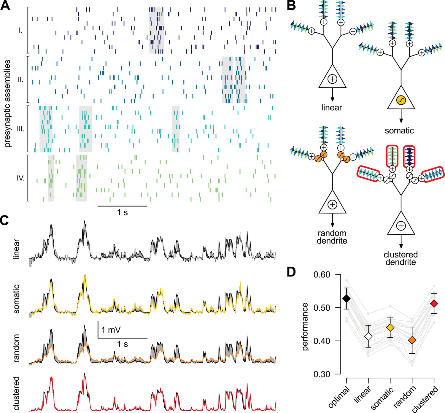
A simple nonlinear dendritic model closely approximates the optimal response for realistic input patterns.
(A) Presynaptic spiking activity matching the statistics observed during hippocampal sharp waves. Spike trains (rows) belonging to four different assemblies are shown (colors), gray shading indicates assembly activations. (B) Different variants of the dendritic model, parts colored in yellow, orange, and red highlight the differences between successive variants (see text for details). (C) Estimating the mean of the presynaptic membrane potentials based on the observed spiking pattern (shown in A) by the optimal response (black) compared to the linear (dotted), somatic (yellow), random (orange) and clustered (red) models. (D) Performance of the four model variants compared to that of the optimal response. Gray lines show individual runs, squares show means.d. Performance is normalized such that is obtained by predicting only the time-average of the signal, and means perfect prediction attainable only with infinitely high presynaptic rates (Materials and methods).
Figure 4—figure supplement 1

Responses of different variants of the dendritic model compared to the true signal.
Responses of different variants of the dendritic model to the spiking pattern shown in Figure 4A of the main paper compared to the true signal (green), that is the mean of the presynaptic membrane potentials. The models shown are the optimal response (A, black) and the linear (B, dotted), somatic (C, yellow), random dendrite (D, orange) and clustered dendrite (E, red) models (see also Figure 4B–D of the main paper). The error (gray areas, measured relative to the signal, cf. Figure 4C where it is measured relative to the optimal response) of the linear, somatic and random models is substantially larger than the error of the optimal response, whereas the response of the clustered model is nearly identical to the optimal response.
Figure 4—figure supplement 2
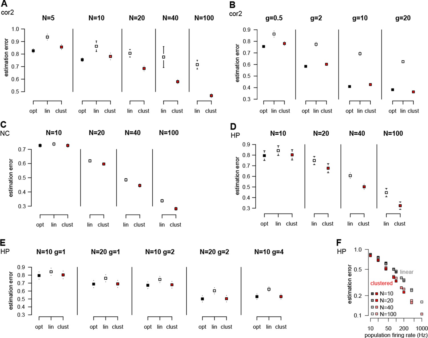
Performance of different neuron models over a wide range of input statistics.
(A) Performance of the optimal (opt) linear (lin) and clustered dendritic (clust) model for presyanaptic statistics with only second-order correlations (Table 1, cor2) with different numbers of presynaptic neurons (), while keeping firing rates fixed ( Hz). (B) Same as (A), but changing firing rates () while keeping the number of presynaptic neurons fixed (at ). The performance of the dendritic neuron is always close to the performance of the optimal response. (With and Hz the dendritic model seems to be slightly better than the optimal response. This is because we derived the optimal response with the assumption that there were no more than one spike in each time bin and we did not enforce this condition in these simulations.) (C) Performance of the models using neocortical input statistics (Table 1, NC) with different numbers of presynaptic neurons. (D) Performance of the models using hippocampal-like input (Table 1, HP; with and ms in D–F) with different numbers of presynaptic neurons. (E) The dendritic model performs significantly better than the linear model and nearly as well as the optimal response for different values of and . (F) The performance of the models depends mostly on the firing rate of the population, , and not on or individually. (Range of values used is shown in the legend, was 1, 2, 4, or 10.) This can be useful because although the computational complexity of the optimal response scales as , and thus computing it for large can be prohibitive, this scaling suggests that, for practical purposes, the large limit can be studied by scaling rather than . Error bars show s.d. and were smaller than the symbols for the means in some cases.
Figure 5 with 2 supplements
Nonlinear dendritic integration is matched to presynaptic input statistics.
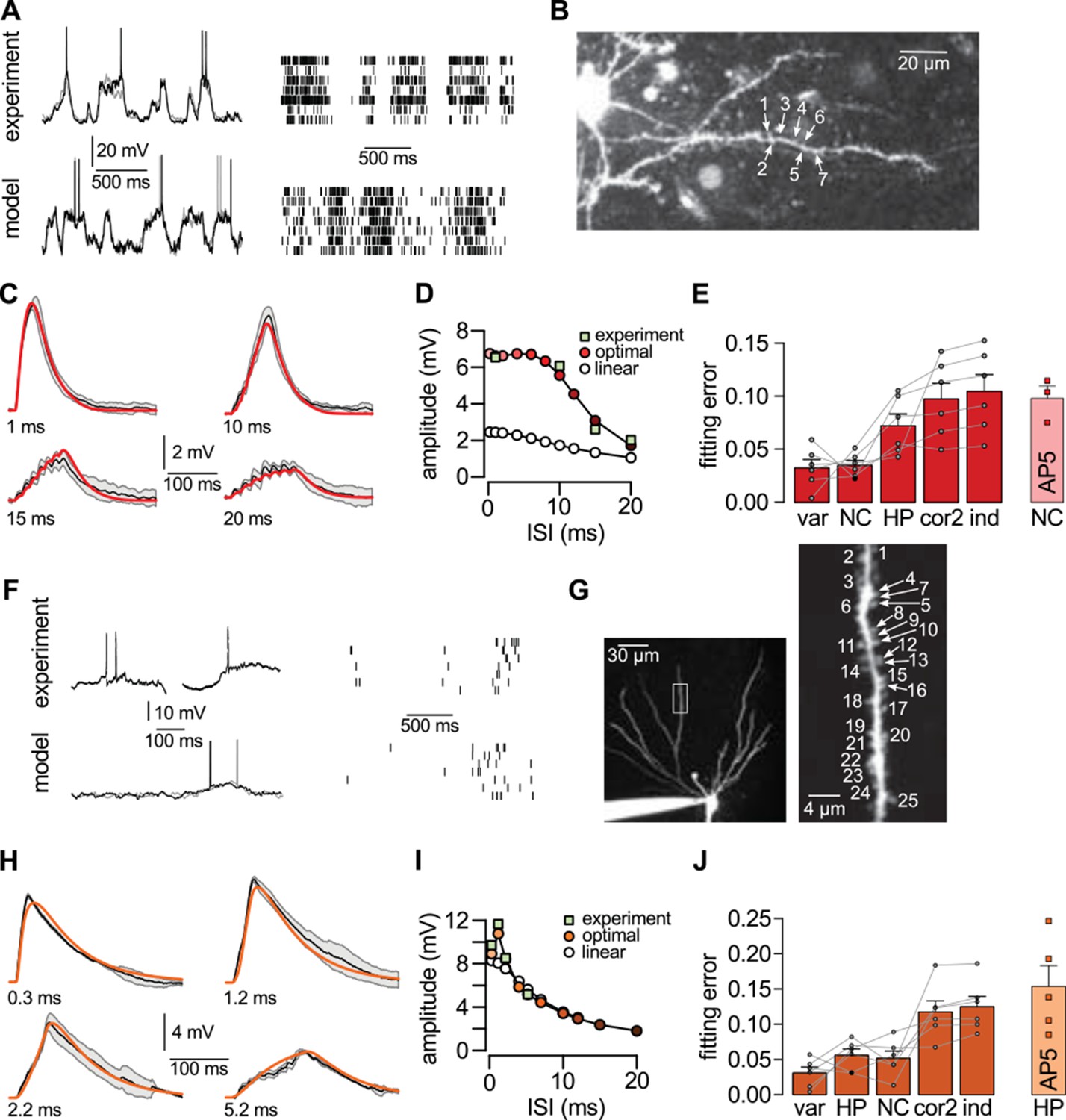
(A) Sample membrane potential fluctuations (left, adapted from Gentet et al., 2010) and multineuron spiking patterns (right, adapted from Ji and Wilson, 2007) recorded from the neocortex (top), and matched in the model (bottom, see also Tables 1–3). (B) Two-photon image of a neocortical layer 2/3 pyramidal cell, numbers indicate individual dendritic spines stimulated in the experiment. (C) Responses to trains of seven stimuli using different inter-stimulus intervals (ISI, shown below traces) recorded in the cell shown in (B) (black; means.d.) and predicted by the optimal response tuned to the presynaptic statistics shown in A (red). Parameters related to postsynaptic dendritic filtering were tuned for the specific dendrite ( Figure 5—figure supplement 1B–C). (D) Dependence of response amplitudes on ISI in the same dendrite shown in B-C (squares), and as predicted by the optimal response (filled circles) or linear integration (empty circles). (E) Average error of fitting dendritic recordings across all dendrites and conditions using the optimal response tuned to different presynaptic statistics (NC, HP, cor2, ind; see text for details) compared to within-data variability (var). Gray lines show individual dendrites. Rightmost bar (NC-AP5) shows fit using NC presynaptic statistics to responses obtained after pharmacological blockade of NMDA receptor activation. (F–J) Same as (A–E) for presynaptic patterns characterized by hippocampal sharp waves (F) and recordings from hippocampal CA3 pyramidal cells (H–J) when stimulating synapses on its basal dendrites (G). In vivo data in (F) was adapted from (Ylinen et al., 1995) (left, membrane potential traces, not simultaneously recorded) and (O'Neill et al., 2006) (right, multineuron spike trains). Error bars show s.e.m.
Figure 5—figure supplement 1

Best fit parameters for fitting dendritic responses.
(A–B) The parameters of the HP and NC models describing the activity of the presynaptic population were fitted to in vivo recordings from the corresponding presynaptic populations (see Materials and methods). When using these presynaptic models to fit individual hippocampal (orange) and neocortical (red) dendritic responses, respectively, we only tuned parameters that characterized the postsynaptic neuron for the optimal response: its membrane time constant, (A), the response amplitude for a single spike (not shown), and the size of the dendritic sububit, i.e. the number of presynaptic neurons innervating a single dendritic branch, (B). (C) When using the cor2 presynaptic model to fit hippocampal (hipp), neocortical (cort) and cerebellar (cbl) dendritic responses, we tuned the correlations between presynaptic neurons, , instead of the size of the dendritic subunit (for an explanation, see also Table 1). Box plots show the range of the data (whiskers), the quartiles (box), and the median (center line). Green lines in (C) show mathematically possible largest negative correlations (), where is the number of presynaptic cells.
Figure 5—figure supplement 2

Dendritic integration in cerebellar stellate cells is not predicted by cortical presynaptic statistics.
We used data recorded from cerebellar stellate cells in which input integration is sublinear (Abrahamsson et al., 2012) to test our predictions with a qualitatively different form of dendritic integration. Stellate cells receive input from cerebellar granule cells (Shepherd, 2004). (A) Top: Presynaptic membrane potential trace recorded intracellularly in a cerebellar granule cell (adapted from Duguid et al., 2012). Bottom: presynaptic membrane potentials in two model neurons (left) and spiking in the model population (right) with simple second-order correlations across cells. (No simultaneously recorded multineural experimental data was available.) Although it is clear from in vivo recordings from cerebellar granule cells that these neurons do not show state-switching dynamics under anesthesia (Duguid et al., 2012), the limited experimental data about their natural population activity made it unfeasible to fit our model quantitatively to data. (B) Responses to increasing number of stimuli (2 10) recorded in a cerebellar stellate cell (black lines, adapted from Abrahamsson et al., 2012) and predicted by the optimal response (thick colored lines) assuming second-order correlations (left) or independence (right) between the membrane potentials of presynaptic neurons. (C) Dependence of response amplitudes on the number of stimuli in the same dendrite shown in (B) (squares, adapted from Abrahamsson et al., 2012), and as predicted by the optimal response (assuming second order correlations, filled circles) or linear integration (empty circles). (D) Average error of fitting dendritic recordings across conditions using the optimal response tuned to different presynaptic statistics (HP, NC, cor2, ind; see main text, and Table 1 for details).
Author response image 1
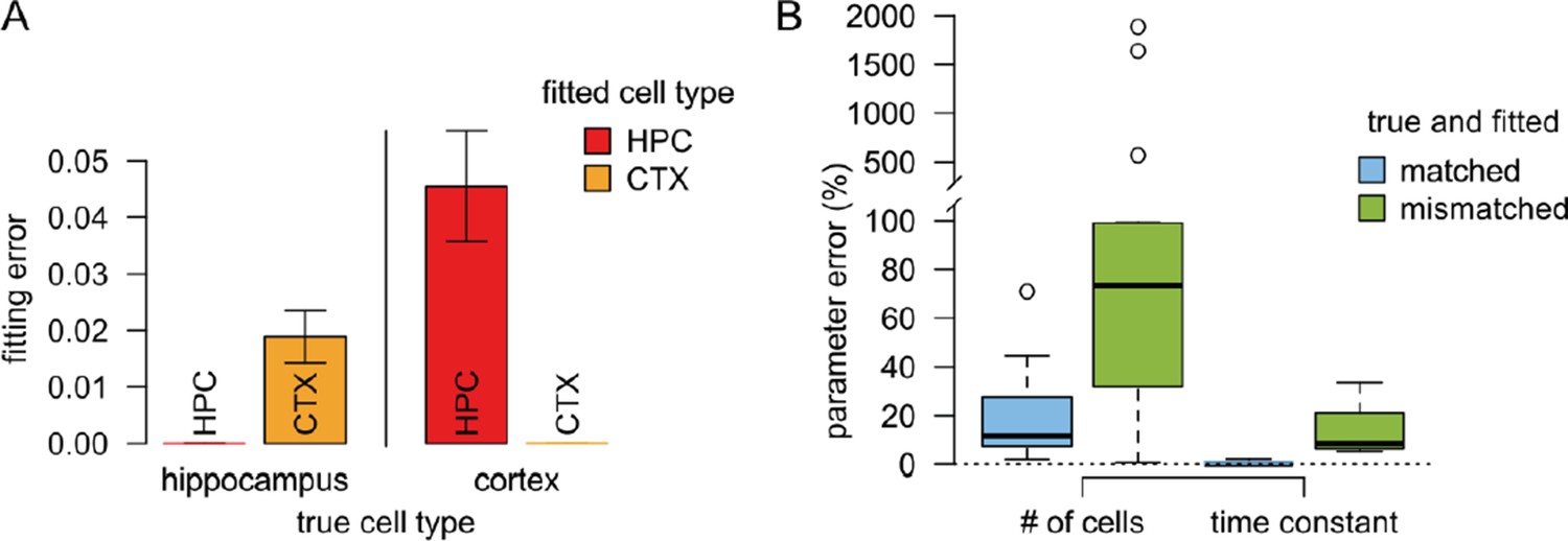
Results of the validation simulations.
(A) The fitting error was substantially smaller if we used similar presynaptic parameters to fit the validation data than the true parameters used to generate the data. In this case the fitting error was essentially zero since there is no intrinsic variability in the artificial data. (B) The error in the postsynaptic parameters (number of cells targeting the dendritic branch, and the postsynaptic filtering time constant) is substantially smaller when the true presynaptic parameters match those used for fitting the model (blue) than when the parameters are mismatched.
Tables
Table 1
Parameters used in Figures 1–5 of the main paper (see also Tables 2–3). () is the rate of switching from the active to the quiescent (from the quiescent to the active) state. The resting potential corresponding to the active and quiescent states is and , respectively. () is the posterior variance (covariance) of the presynaptic membrane potential fluctuations in a given state where . τrefr is the length of the refractory period and is the baseline transmission probability in these synapses (13, 49).
| Figure 1 | Figure 2 | Figure 3 | Figure 4 | Figure 5 | |||||||
|---|---|---|---|---|---|---|---|---|---|---|---|
| parameter | unit | B,C | A,B | C,D | A | B | A-D | ind | cor2 | NC | HP |
| Hz | 10 | – | 10 | 10 | – | 10 | – | – | 10 | 10 | |
| Hz | 10 | – | 0.27 | 0.67 | – | 0.67 | – | – | 4 | 0.027 | |
| mV | 2.4 | 0 | 2.3 | 2.3 | 0 | 2.3 | 0 | 0 | 10 | 2.3 | |
| ms | 20 | 20 | 20 | 20 | 20 | 20 | 20 | 20 | 20 | 20 | |
| mV | 1 | 16 | 4 | 1 | 1 | 1 | 1 | 1 | 10 | 1 | |
| mV | 0 | 0.5 | 0.5 | 0 | 0.5 | 0 | 0 | * | 5 | 0.5 | |
| Hz | 1 | 1 | 1 | 5.3 | 0.5 | 5 | 0.5 | 0.5 | 1 | 2 | |
| mV | 1 | 0.4 | 0.4 | 0.5 | 0.4 | 0.4 | 1 | 2 | 0.1 | 0.6 | |
| ms | 3 | 3 | 3 | 1 | 3 | 1 | 3 | 3 | 3 | 3 | |
| – | 1 | 1 | 1 | 1 | 1 | 1 | 1 | 1 | 0.5 | 0.2 | |
| – | 20 | 70 | 20 | 10 | 10 | 10 | +0† | +20† | * | * | |
| ms | 0 | 10 | 10 | 0 | 0 | 0 | * | * | * | * | |
| – | * | * | * | * | |||||||
-
*These parameters were fitted to experimentally recorded dendritic responses, see Figure 5—figure supplement 1. †The numbers 0 and 20 indicated here are in addition to the number of stimulated synaptic sites in the experiment. For the ind model, this number does not affect the predictions, for the cor2 model its effects could phenomenologically be incorporated into which we chose to fit instead.
Table 2
Features of neocortical population activity during quiet wakefulness. Parameters of the model are given in column NC of Table 1.
| Data | Model (NC) | Reference | |
|---|---|---|---|
| duration of active states | 130 ms | 100 ms | Gentet et al. (2010) |
| duration of quiescent states | 200 ms | 250 ms | Gentet et al. (2010) |
| , firing rate during active states | 2.5 Hz | 2.86 Hz | Gentet et al. (2010) |
| , firing rate during quiescent states | 1/3 Hz | 0.39 Hz | Gentet et al. (2010) |
| , depolarisation during active states | 20 mV | 20 mV | Gentet et al. (2010) |
| time constant | 20 ms | 20 ms | Poulet and Petersen (2008) |
Table 3
Features of hippocampal population activity during sharp wave-ripple states. Parameters of the model are given in column HP of Table 1A recent intracellular study (English et al., 2014) recording from CA1 neurons in awake mice found parameters similar to our previous estimates. Using the parameters found in that study – Hz, Hz (Table 1 of English et al., 2014), mV and mV (Figure 3A of English et al., 2014) yielding Hz and mV – did not influence our results (not shown).
| Data | Model (HP) | Reference | |
|---|---|---|---|
| activation rate of an ensemble | 0.25 Hz | 0.027 Hz | Grosmark et al. (2012); Pfeiffer and Foster (2013) |
| duration of SPWs | 105 ms | 100 ms | Csicsvari et al. (2000) |
| , firing rate during SPW | 10 Hz | 9.5 Hz | Csicsvari et al. (2000) |
| , firing rate between SPWs | 0.5 Hz | 0.6 Hz | Grosmark et al. (2012); Csicsvari et al. (2000) |
| , depolarisation during SPWs | 0–10 mV | 4.6 mV | Ylinen et al. (1995) |
| time constant | 8–22 ms | 20 ms | Epsztein et al. (2011) |
Download links
A two-part list of links to download the article, or parts of the article, in various formats.
Downloads (link to download the article as PDF)
Open citations (links to open the citations from this article in various online reference manager services)
Cite this article (links to download the citations from this article in formats compatible with various reference manager tools)
Dendritic nonlinearities are tuned for efficient spike-based computations in cortical circuits
eLife 4:e10056.
https://doi.org/10.7554/eLife.10056


